Long Write-Up

The Fitter is designed to be used for SANS data processing first of all. Thus, SANS theoretical models are implemented in it. Moreover, some standard mathematical models are added for wider applicability. Besides the implemented theoretical models, Fitter has a minimization module. It provides a safe call of MINUIT [25] procedures in the current version. The important feature of Fitter's design is its expandability: both new models and new minimizing algorithms can easily be added to the existing ones.

Theoretical Models

Fig. 1: Fitter's model module class hierarchy

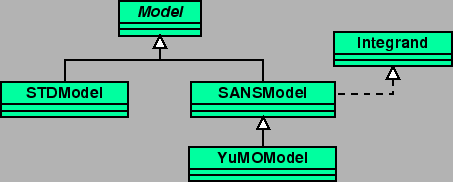
Fitter's model module is designed as follows (fig.1). Abstract base class Model provides a common interface, used by a minimization module. Thus, any theoretical model class inherits from it. Model classes currently implemented in the Fitter are: STDModel, SANSModel, YuMOModel. Each concrete class provides several theoretical functions. All of them are described below.

Standard Models

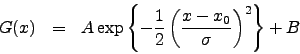
Standard mathematical models implemented in the Fitter are:

• Gaussian
  $$\begin{eqnarray*} G(x) &=& A \exp\left\{-\frac{1}{2}\left(\frac{x-x_0}{\sigma}\right)^2\right\} + B \end{eqnarray*}$$
  
  

• Exponential
  $$\begin{eqnarray*} E(x) &=& A \exp\left\{mx+b\right\} + B \end{eqnarray*}$$
  
  

• Polynomials up to the eighth order
  $$\begin{eqnarray*} P_n(x) &=& \sum\limits_{k=0}^{n}p_k x^k \end{eqnarray*}$$
  
  

SANS (Small-Angle Neutron Scattering) Models

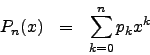
Determination of invariants for small-angle scattering curves allows one to analyze the structure of a particle under study. Upon the first step of this analysis the particle form is approximated by simple geometrical bodies - ellipsoids, cylinders, prisms.

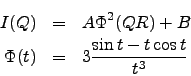
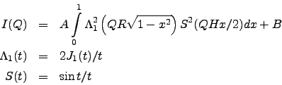
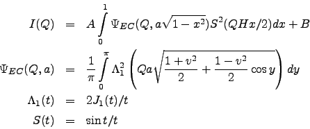
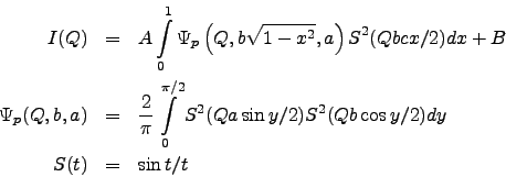
Thus, SANS models implemented in the Fitter are:

• Ball of the radius $R$
  $$\begin{eqnarray*} I(Q) &=& A \Phi^2(QR) + B \\ \Phi(t) &=& 3\frac{\sin t-t\cos t}{t^3} \end{eqnarray*}$$
  
  

• Ellipsoid of revolution with half-axises $a$ and $av$
  $$\begin{eqnarray*} I(Q) &=& A \int\limits_{0}^{1} \Phi^2\left[ Qa\sqrt{1+x^2(v^2-1)} \right] dx + B \\ \Phi(t) &=& 3\frac{\sin t-t\cos t}{t^3} \end{eqnarray*}$$
  
  

• Cylinder of the radius $R$ and the length $H$
  $$\begin{eqnarray*} I(Q) &=& A \int\limits_{0}^{1} \Lambda_1^2\left(QR\sqrt{1-x^... ... dx + B \\ \Lambda_1(t) &=& 2J_1(t) / t \\ S(t) &=& \sin t / t \end{eqnarray*}$$
  
  

• Elliptical cylinder with half-axises $a$, $av$ and the length $H$
  $$\begin{eqnarray*} I(Q) &=& A \int\limits_{0}^{1} \Psi_{EC}(Q,a\sqrt{1-x^2}) S^... ...ght) dy \\ \Lambda_1(t) &=& 2J_1(t) / t \\ S(t) &=& \sin t / t \end{eqnarray*}$$
  
  

• Parallelepiped with the ribs $a$, $b$, $c$
  $$\begin{eqnarray*} I(Q) &=& A \int\limits_{0}^{1} \Psi_p\left(Q,b\sqrt{1-x^2},a... ...i/2} S^2(Qa\sin y/2) S^2(Qb\cos y/2) dy \\ S(t) &=& \sin t / t \end{eqnarray*}$$
  
  

• Spherical shell of the outer radius $R_{1}$ and the inner radius $R_{2}$
  $$\begin{eqnarray*} I(Q) &=& A \left[ \Phi(QR_1)-\left(\frac{R_2}{R_1}\right)^3\Phi(QR_2) \right]^2 + B \\ \Phi(t) &=& 3\frac{\sin t-t\cos t}{t^3} \end{eqnarray*}$$
  
  

More detailed information about SANS models is available in [22].

SANS Models with YuMO spectrometer resolution

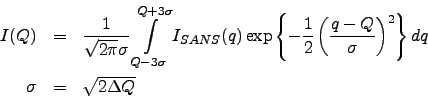
These models are implemented to fit data measured on the YuMO spectrometer [23] operated on the 4-th channel of the fast pulsed reactor IBR-2 [24]. YuMO models are the same as SANS, but they take into account the spectrometer resolution.

• SANS Model with resolution
  $$\begin{eqnarray*} I(Q) &=& \frac{1}{\sqrt{2\pi}\sigma} \int\limits_{Q-3\sigma}^... ...q-Q}{\sigma}\right)^2\right\} dq \\ \sigma &=& \sqrt{2\Delta Q} \end{eqnarray*}$$
  
  

Minimization

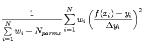
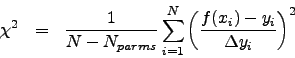
To find theoretical model parameters, one should minimize a functional, which is a measure of deviation between a theoretical curve and experimental data. In a common case of a least-squares fit, the functional under minimization is a chi-square:

$$\begin{eqnarray*} \chi^2 &=& \frac{1}{N-N_{parms}} \sum\limits_{i=1}^{N} \left(\frac{f(x_i)-y_i}{\Delta y_i}\right)^2 \end{eqnarray*}$$

Minuit

We are using ROOT::TMinuit class to perform a minimization. This package was originally written in Fortran by Fred James and part of PACKLIB (patch D506) and has been converted to a C++ class by R.Brun. The current implementation in C++ is a straightforward conversion of the original Fortran version. The main changes are:

• The variables in the various Minuit labeled common blocks have been changed to the TMinuit class data members.
• The internal arrays with a maximum dimension depending on the maximum number of parameters are now data members arrays with a dynamic dimension such that one can fit very large problems by simply initializing the TMinuit constructor with the maximum number of parameters.
• The include file Minuit.h has been commented as much as possible using existing comments in the code or the printed documentation
• The original Minuit subroutines are now member functions.
• Constructors and destructor have been added.
• Instead of passing the FCN function in the argument list, the addresses of this function is stored as pointer in the data members of the class. This is by far more elegant and flexible in an interactive environment. The member function SetFCN can be used to define this pointer.
• The derived class TMinuitOld contains obsolete routines from the Fortran based version.

Additional modifications were made to separate TMinuit class from the ROOT package (Fitter is ROOT independent indeed).

MINUIT offers the user a choice of several minimization algorithms. The MIGRAD algorithm is, in general, the best minimizer for nearly all functions. It is a variable-metric method with inexact line search, a stable metric updating scheme, and checks for positive-definiteness. Its main weakness is that it depends heavily on knowledge of the first derivatives, and fails miserably if they are very inaccurate.

For further details see MINUIT documentation [25].

Robust Fitting

The least-squares fitting involves the minimization of the sum of the squared residuals. There are two instances where this minimization produces less than satisfactory fit:

1. The significant outliers are present in data. In this case, the square of the residuals of these out-lier points may, within a given region, significantly shift the fitted curve away from the bulk of the data.
2. The the Y-data span more than several orders of magnitude. The squared residuals of the largest valued Y-points can overwhelm the influence of the squared residuals of the smallest Y-valued points, causing the smallest Y-value points to either be poorly fitted or not fitted at all. Data that require a logarithmic Y-scale to see all of the points may be a good candidate for robust fitting, especially if four or more major log divisions take place.

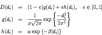
Robust estimates designed to be successful in such cases. The essence of robust fitting is to use a minimization that is less influenced by outliers and the dynamic range of the Y-variable. Each data measured point took into account with it own weight, which indicate influence of given point.

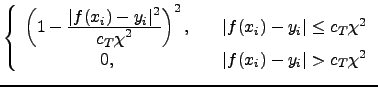
It is based on so-called M-estimates which follow from maximum like-hood approach, M-estimates are usually the most relevant for model fitting. Robust approach uses gross-error model (Hubert). Probability distribution function of measurement errors $d_{i}$ suggested as a superposition of two distributions: basic $g(d_{i})$ and distribution of big errors $h(d_{i})$

$$\begin{eqnarray*} D(d_i) &=& (1-\epsilon)g(d_i) + \epsilon h(d_i), \quad \epsilo... ... h(d_i) &=& \alpha \exp \left\{ -\beta \vert d_i\vert \right\} \end{eqnarray*}$$

In practice, robustness works also in cases of other distributions $h(d_{i})$, for example, normal one like $g(d_{i})$ is, but with bigger RMS.

Application of maximum like-hood approach and few simplifications and the fact that RMS of the distribution $g(d_{i})$ can be approximated by chi-square of data points, give us well known Tukey bi-square weights, which is suitable in most cases.

$$w_i = \left\{ \begin{array}{cr} \left(1-\frac{\displaystyle \vert f(x_i... ... c_T \chi^2 \\ 0, \quad &\vert f(x_i)-y_i\vert > c_T \chi^2 \end{array}\right.$$ (1)

In chi-square function data values are multiplied by their weights:

$$\chi^2 = \frac{1}{\sum\limits_{i=1}^{N}w_i - N_{parms}} \sum\limits_{i=1}^{N} w_i \left(\frac{f(x_i)-y_i}{\Delta y_i}\right)^2$$ (2)

The initial values of the weights are equal to 1. In the following iterations, weights are recalculated after each procedure of minimization and calculation of the new value of chi-square. Iterations are repeated until convergence (until chi-square value is stabilized within a predefined accuracy).

In general, the robust approach looks like:

• setting $w_i=1$, calculating $\chi^2$ by (2), setting $c_T = 5$;
• while $c_T > 1$ doing the loop:
  • calculating $w_i$ by (1) using current values of $\chi$ and $c_T$;
  • minimizing $\chi^2$ given by (2);
  • reducing $c_T$ by $c_T/=2$.

For detailed explanation see [26,27,28].