Examples

Robust feature example

Here is a simple example of the Robust feature usage. File test.dat is an example of input data for fitter. It is just a generated gaussian distribution, contaminated by uniformly distributed random noise.

Typing in command line

% fitter test.dat -o fit1.dat --std g 

we get the following result:

____________________________________________________
Model.......................................Gaussian
____________________________________________________
Mean.............................-0.4576 +- 0.1719
RMS...............................1.7571 +- 0.3680
Amplitude.........................7.1333 +- 0.5719
Background.......................17.3032 +- 0.6111
____________________________________________________
Chi square....................................1.1068
____________________________________________________

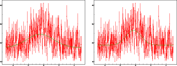
and the fitting curve shown in fig.3 (left).

Fig. 3: Highly noisted data fitting example

This fit is not good enough, thus, we try

% fitter test.dat -o fit2.dat --std g -r

invoking robust fitting. This gets a better result:

____________________________________________________
Model.......................................Gaussian
____________________________________________________
Mean.............................-0.2564 +- 0.1595
RMS...............................0.9985 +- 0.1638
Amplitude.........................7.8680 +- 1.2633
Background.......................18.6319 +- 0.5641
____________________________________________________
Chi square....................................1.0708
____________________________________________________

The fitting curve (fig.3, right) is much better this time.

SANS/YuMO example

To demonstrate the fitter usage, we have used the results of neutron measurements, obtained on the apoferritin protein sample obtained from Aldrich corporation. The file apdn.dat containing a SANS spectra is used as fitter input. A spherical shell model, which is one of the most adequate for apoferritin, is chosen. The corresponding command line is the following:

% fitter apdn.dat -o apdn.fit --yumo ss

This gives the following result:

____________________________________________________
Model................Spherical shell with resolution
____________________________________________________
Outer radius.....................59.6547 +- 0.0576
Inner radius.....................40.1314 +- 0.0700
Amplitude........................28.3414 +- 0.1721
Background........................0.0191 +- 0.0003
____________________________________________________
Chi square...................................31.2243
____________________________________________________

and the fitting curve shown in fig.4.

Fig. 4: Apoferritin data fitting example