|
|
|

|
PROGRAM LIBRARY JINRLIBOPEM2 - orthonormal polynomial expansion method in two dimensions and its realization in fortran packageAuthor: Nina B.Bogdanova Institute of Nuclear Research and Nuclear Energy, Sofia, Bulgaria |
|
|

|
|
Language: Fortran 77, Windows A package of Fortran 77 programs is presented. This package has developed since 1981 for the calibration problems of measurement devices in High Energy Physics in collaboration with LIT JINR, Dubna. Last version of the package is developed in part under the contract of Bulgarian National Council for Sientific Research - Phi 1001.
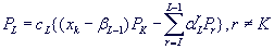
1.Description of the Method Orthonormal Polynomial Expansion Method (OPEM2) is the method of orthogonalization of polynomials based on Householder-Forsythe 3-term relation [1,2] (one-dimensional case) and the Weisfeld recurrence [3] (many-dimensional case). The recurrence family of polynomials {PL} is given by:
where Pk is a mother term. K and I have to be determined. {PL}
are defined in a finite discrete subset D of
Then orthonormal coefficients {ak} in (1.2) are easily computed by given values:
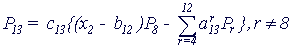
A pyramid of two-dimensional polynomials is given - the hierarchy order of polynomials in two variables: 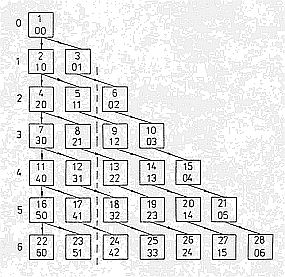 In the cell on the top the number of polynomial is given, and the degrees j1 and j2 of the x1 and x2 variables also - on the bottom. One example for evaluating K and I in (1.1) gives for the polynomial P13 (k=2, j1=2, j2=2):
(P8 is a mother term: K=8, I=4). New theoretical investigations are presented in two-dimensional case in [7] for the case of differentiation and integration - the fourth member in the equation (1.1) is added. More detailed description of the mathematical method with many-dimensional polynomials including differentiation and integration will be published later in suitable journal according the description in JINR library with some implementations.
2.Description of the package OPEM2 (fortran 77) It consists of main program CALIB and five subroutines: the principle TSTWO, ORTTWO, PRETWO and 2 auxiliary DEGREE, NUMBER. The main program CALIB gives:
The principal subroutines contain a named common /LINKS/ where the recurrence factors and auxiliary variables are recorded. The present size of /LINKS/ allows for overall degrees as high as 16 and for Lmax=(16+1)(16+2)/2=153. The array dimensions in /LINKS/ may be changed.
The subroutine TSTWO(X,Y,W,M,F,A,NDEG) is the subroutine,
which calls subprograms. First, it calls PRETWO for preparing
the recurrence factors with overall degree NDEG. Afterwards it
calculates the orthonormal coefficients A, calling the subroutine
ORTTWO. After second call of ORTTWO it calculates the approximating
values and deviations in the points, selects optimal degree Lr,
selects min (
The subroutine ORTTWO(NUMBMX,X,Y,POLY) returns the specific values of all polynomials in an orthonormal series from 1 to NUMBMX at given values of x and y in POLY-array.
The subroutine PRETWO(M,MAXD,X,Y,W,POLY) prepares the recurrence factors of two-dimensional polynomials, orthonormal over a discrete point set in a single call, which must precede any working call of ORTTWO.
PRETWO makes successive recursive calls to ORTTWO with NUMBMX = L-1, then L is incremented, etc, until Lmax is reached. The subroutine DEGREE(N,J,JX,JY) calculates at given ordinary number of polynomials N the overall degree of the leading term J, the degree in x-variable JX, and that in y-variable JY. The integer function NUMBER(JX,JY) at given x degree JX and y degree JY returns the ordinary number of polynomials in a series according to Weisfeld [3] with particular stress on the leading term.
3.Applications Some applications for receiving calibration coefficients between ideal and measured grid in the optical devices in HEP are given in [5,6,7]. The last application of the package is for H1 experiment in DESY, Hamburg - to look for the coordinates of the maximum of the surface formed by gaussians. The analytic surface over the 400 point's grid is our approximation. It is done in collaboration with Dubna (LIT). 4.References
Sources of OPEM2 are submitted. 


|
|
 , D={q1,q2,...,qM}.
Every point qj=qj(x1j1,x2j2,...,xnjn) presents a n-coordinate vector
(in this case n=2). The weights, associated with them, wj=1/S2j,
depend on the standard deviation in every point. The points, the weights
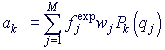
and the experimental function values {qj,wj,fjexp}j=1M are given. The recurrence coefficients {
, D={q1,q2,...,qM}.
Every point qj=qj(x1j1,x2j2,...,xnjn) presents a n-coordinate vector
(in this case n=2). The weights, associated with them, wj=1/S2j,
depend on the standard deviation in every point. The points, the weights
and the experimental function values {qj,wj,fjexp}j=1M are given. The recurrence coefficients { L} and {
 L-1} and normalizing factor {cL}
are evaluated by scalar products of the given values. The description
here follows the descriptions [3,4,7]. In OPEM2 the approximated function
is given by the expansion of the orthonormal polynomials using special
orthonormal coefficients ak. Optimal value of polynomial degree - Lr
is evaluated using two criteria.
L-1} and normalizing factor {cL}
are evaluated by scalar products of the given values. The description
here follows the descriptions [3,4,7]. In OPEM2 the approximated function
is given by the expansion of the orthonormal polynomials using special
orthonormal coefficients ak. Optimal value of polynomial degree - Lr
is evaluated using two criteria.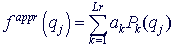
 )2, calculates the errors of series coefficients
after third call of ORTTWO and then prints the results.
)2, calculates the errors of series coefficients
after third call of ORTTWO and then prints the results.