Lifting scheme

The purpose of this section is to give a brief description of the lifting scheme. A more detailed information can be found in [4,5].

Constructing wavelets using lifting consists of three simple phases. The first step or Lazy wavelet splits the data $\{\lambda_{0,k}\}$ into two subsets, even and odd. The new data sequence is given by

$$\lambda_{-1,k} = \lambda_{0,2k} \,\, , \quad k\in \mathbf{Z} \,\, ,$$ (1)

and coefficients

$$\gamma_{-1,k} = \lambda_{0,2k+1} \,\, , \quad k\in \mathbf{Z} \,\, ,$$

encode the difference between $\{\lambda_{0,k}\}$ and $\{\lambda_{-1,k}\}$. We refer to them as wavelet coefficients.

The second step calculates the wavelet coefficients (high pass) as the failure to predict the odd set based on the even:

$$\gamma_{-1,k} = \gamma_{-1,k} - P(\lambda_{-1,k}) \,\, .$$ (2)

A simple example of (2) is

$$\gamma_{-1,k} = \gamma_{-1,k} - (\lambda_{-1,k} +\lambda_{-1,k-1}) / 2 \,\, ,$$

i.e. $P$ is a function piecewise linear over intervals of length 2, and wavelet coefficients measure to which extent the original signal fails to be linear. In terms of frequency content, the wavelet coefficients capture high frequencies in the original signals. The prediction does not necessary to be linear. We could try to find the failure to be cubic and any other higher order [4,5].

For our practical purpose we use the cubic interpolation scheme, using two neighboring values on either side and define the (unique) cubic polynomial which interpolates those four values. This interpolation scheme allows us to easily accommodate interval boundaries for finite sequences, such as in our case. For the cubic construction described above, we can take 1 sample on the left and 3 on the right at the left boundary of an interval. The cases are similar if we are at the right boundary.

Finally, the third step updates the even set using the wavelet coefficients (low pass). The idea is to find a better $\lambda_{-1,k}$ so that a certain scalar quantity $Q()$, i.e. mean, is preserved, or

$$Q(\lambda_{-1,k}) = Q(\lambda_{0,k}) \,\, .$$

We construct an operator $U$ and update $\{\lambda_{-1,k}\}$ as

$$\lambda_{-1,k} = \lambda_{-1,k} + U(\gamma_{-1,k}) \,\, .$$ (3)

In a simple case, for a long signal, we can update the $\lambda$ coefficients with the following equation:

$$\lambda_{-1,k} = \lambda_{-1,k} + (\gamma_{-1,k} + \gamma_{-1,k-1}) / 4 \,\, .$$

We choose the updating operator $U$ so that 3 moments of the $\lambda$'s at every level are preserved (see [4,5] for details).

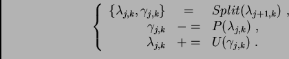
The three stages of lifting described by (1), (2) and (3) are combined and iterated to generate the fast lifted wavelet transform algorithm:

$$\left\{ \begin{array}{rcl} \{\lambda_{j,k}, \gamma_{j,k}\} & ... ... \lambda_{j,k} & += & U(\gamma_{j,k}) \,\, . \end{array}\right.$$

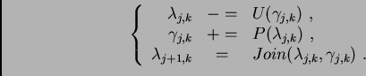
We can now illustrate one of the nice properties of lifting: once we have the forward transform, we can immediately derive the inverse. We just have to reverse the operations and toggle $+$ and $-$. This idea leads to the following inverse transform:

$$\left\{ \begin{array}{rcl} \lambda_{j,k} & -= & U(\gamma_{j,k... ...= & Join(\lambda_{j,k}, \gamma_{j,k}) \,\, . \end{array}\right.$$

An example with using the filter coefficients $(1/2,1/2)$ (at the predict stage) and lifting coefficients $(1/4,1/4)$ (at the update stage) already shows how the lifting scheme can speed up the implementation of the wavelet transform. Classically, the $\{\lambda_{-1,k}\}$ coefficients are found as the convolution of the $\{\lambda_{0,k}\}$ coefficients with the filter $\tilde h = \{ -1/8, 1/4, 3/4, 1/4, -1/8\}$. This step would take 6 operations per coefficient while lifting only needs 3.

The total number of iterations in this simplest case is $n=\left[\log_2\left(L-1\right)\right]$, where $L$ is the signal length. In the case we use $$n=\left[\log_2\left(\frac{L-1}{3}\right)\right]$$. It can be seen from this equation that the size of the signal does not matter, i. e., signals do not necessarily have to have dyadic dimensions. The interpolating subdivision guarantees a correct treatment of the boundaries for every case.