4.1.1 Continuous WT |
( Next Previous Contents ) |
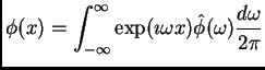
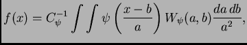
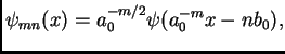
Formally, the wavelet transform of a function
![]() 2is a projection of
2is a projection of ![]() to the basic wavelet
to the basic wavelet ![]() dilated by factor
dilated by factor ![]() and
shifted by
and
shifted by ![]() :
:
![[*]](crossref.png) ) into
() and making Fourier transform
) into
() and making Fourier transform
 ),
if the function
),
if the function
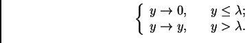
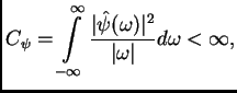
The admissibility condition (), which provides a possibility
of a function ![]() to be used as a basic wavelet
to be used as a basic wavelet ![]() , is rather loose.
That is why there exist a lot of different basic wavelets invented
by Daubechies [6], Meyer [7], Mallat
and others [8].
, is rather loose.
That is why there exist a lot of different basic wavelets invented
by Daubechies [6], Meyer [7], Mallat
and others [8].
4.1.1.1 Gaussian wavelets |
( Next Previous Contents ) |
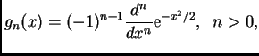
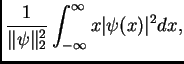
Amongst all differentiable functions used as wavelets, the derivatives of the Gaussian
).
It follows from the definition () that
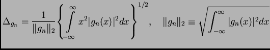
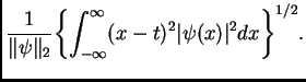
The localization properties for ![]() family can be evaluated explicitly.
In general case the continuous wavelet transform with basic wavelet
family can be evaluated explicitly.
In general case the continuous wavelet transform with basic wavelet
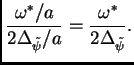
![]() is centered at
is centered at ![]() and has the window width
and has the window width
![]() :
:
![$\displaystyle \left[ \frac{w^*}{a} - \frac{1}{a}\Delta_{\tilde\psi},
\frac{w^*}{a} + \frac{1}{a}\Delta_{\tilde\psi} \right] \,\, .
$](img35.png) ). Using the
definition ():
). Using the
definition ():
| Wavelet | Window width | |
|
|
|
|
|
|
|
4.1.1.2 Examples |
( Next Previous Contents ) |
As the first example of how wavelets work, let us take a harmonic signal
constructed by superposing the low-frequency one with the small
fraction of the high-frequency one and then contaminating it by
uniformly distributed random noise, see Fig. .
|
Let us perform ![]() -wavelet transform (widely known as "Mexican hat") of the
contaminated signal.
Fig. (left) presents the
wavelet spectrum.
The shade-plot provides a powerful tool,
which helps to display the
structure of the signal. The set of wavelet coefficients can be presented
as a projection of 3-dimensional surface
-wavelet transform (widely known as "Mexican hat") of the
contaminated signal.
Fig. (left) presents the
wavelet spectrum.
The shade-plot provides a powerful tool,
which helps to display the
structure of the signal. The set of wavelet coefficients can be presented
as a projection of 3-dimensional surface ![]() onto the
onto the ![]() -
-![]() plane.
Coefficients with higher values are shown in light colors,
the lower ones in dark.
Although the wavelet spectrum is very informative, it often brings too much
visually redundant information.
To make it more contrast, the gray-scaled image is often
transformed to the so-called wavelet skeleton.
Lines on the skeleton correspond to local maxima of the wavelet coefficients.
plane.
Coefficients with higher values are shown in light colors,
the lower ones in dark.
Although the wavelet spectrum is very informative, it often brings too much
visually redundant information.
To make it more contrast, the gray-scaled image is often
transformed to the so-called wavelet skeleton.
Lines on the skeleton correspond to local maxima of the wavelet coefficients.
|
In the next figure the results of the final ![]() -filtering of the same signal
are shown.
First, we accomplish
-filtering of the same signal
are shown.
First, we accomplish ![]() -filters with four selected scales only: 32, 64, 128
and 256. The result of the inversion is the signal in fig. a.
When our signal was processed at scales 1, 2, 4, 8 and 16 its inversion gives
result in Fig. b.
-filters with four selected scales only: 32, 64, 128
and 256. The result of the inversion is the signal in fig. a.
When our signal was processed at scales 1, 2, 4, 8 and 16 its inversion gives
result in Fig. b.
|
It is seen that the filter allows to extract both components of the original signal. Thus selecting properly the scales of the wavelet transformation it is possible to highlight the components of desired scales. It should be pointed out here, that with the same signal the simple Fourier filter would fail. It could be done, in principle, as well by applying a Fourier filter, but as two-step procedure: to select the high frequency short-living sin-wave you should, first, extract the low-frequency wave and than subtract it from the signal. The wavelet filter allows a direct extraction of the desired component.
![\includegraphics[width=6cm]{fig/e10-2001-205/CWT/skel05.eps}](img54.png)
|
Another important application of wavelets is signal denoising. The
procedure of denoising consists of nullifying wavelet
coefficients with small amplitude before inverse
transform. The ![]() skeleton of the signal after such denoising
is shown in Fig. .
As one can see, its typical high-frequency part
produced by noise is efficiently suppressed. Then the inverse transform
would enhance the corrupted signal back to its original view in
Fig. a.
skeleton of the signal after such denoising
is shown in Fig. .
As one can see, its typical high-frequency part
produced by noise is efficiently suppressed. Then the inverse transform
would enhance the corrupted signal back to its original view in
Fig. a.
4.1.1.3 Implementation in WASP |
( Next Previous Contents ) |
The direct evaluation of the convolution in the direct () and
inverse () wavelet transform may be performed numerically but is
expensive in memory and CPU time. At the same time, the self-similarity
property of WT suggests the methods for constructing
fast and effective algorithms.
The straightforward way of WT
implementation is to restrict the calculation on a discrete
sub-lattice
An inverse discrete transform
 ).
).
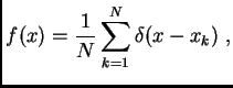
However,
if the analyzed signal consists of a discrete set of measured counts
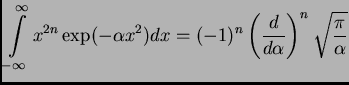
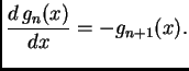
![]() , we can realize two discretization schemes
using the explicit integration formula of explicit integration
of Gaussian wavelets over bins to speed up the computations.
, we can realize two discretization schemes
using the explicit integration formula of explicit integration
of Gaussian wavelets over bins to speed up the computations.
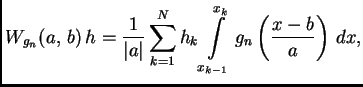
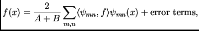
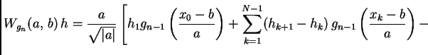
For a discretized signal
) is written as
) is nothing but the ``averaged sum'' of the wavelets
The formula () does not contain integral and this fact allows one
to speed-up the wavelet transform algorithm for discretized signals like
().
Thus, () is just what is used in WASP for the wavelet analysis.
However for gaussian wavelets (GW) especially there is one more
way to improve this algorithm [5].
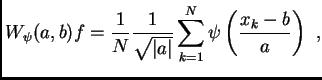
Having a discretized signal
![]() ,
one can define
,
one can define
Due to () we can replace the integral by the difference
).
However this expression is still rather slow to evaluate and could be used
only for obtaining a few coefficients.
For example, applying () to
calculate
![]() while
while ![]() is fixed, but
is fixed, but ![]() runs over
runs over
![]() values
values
![]() ,
,
![]() one needs to
calculate
one needs to
calculate ![]() values of the wavelet
values of the wavelet ![]() in points
in points
![]() .
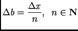
Nevertheless, if we restrict the choice of the shift steps, as
.
Nevertheless, if we restrict the choice of the shift steps, as
) to calculate
).
Thus we consider the values of 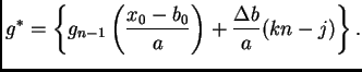
In the second case () one has the vector
![]() with
with ![]() components and should replace
everywhere
components and should replace
everywhere ![]() and
and ![]() by
by ![]() and
and ![]() .
.
The next substantial resource of increasing the speed of calculations is based on the practically compact support of the GW in space.
4.1.2 Discrete WT |
( Next Previous Contents ) |
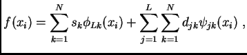
The main idea of a discrete wavelet transform is to represent a given data as
a decomposition using basis functions
![]() ,
,
![]() .
They are constructed as scaled and shifted two basic functions:
.
They are constructed as scaled and shifted two basic functions:
 |
.
Each decomposition step realized by using two filters: ![]() -- low pass
filter and
-- low pass
filter and ![]() -- high pass filter.
Filters
-- high pass filter.
Filters ![]() and
and ![]() depend on functions
depend on functions ![]() and
and ![]() as follows:
as follows:
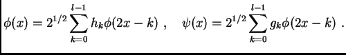 |
shows one decomposition step.
4.1.3 Data filtering |
( Next Previous Contents ) |
The filtering is carried out in three steps:
One of the useful properties of WT is its ability to denoise a data by thresholding. There are two basic methods yielding a good result:
 |
.
4.1.4 Lifting scheme |
( Next Previous Contents ) |
Follow W.Sweldens [11], let us assume that we have a signal and
we need to make a decomposition of this signal into a non-correlated parts.
First we separate the signal into a two equal parts, by putting all even
points into one array, and all odd into another.
If the data in the source signal are correlated, than the first array
contains some information about the second one. Let us denote these two
arrays by ![]() and
and ![]() , respectively. Thus the first stage
of the lifting scheme is two separate data into two classes.
The second stage of the lifting scheme is
to find a data-independent prediction
operator, such that
, respectively. Thus the first stage
of the lifting scheme is two separate data into two classes.
The second stage of the lifting scheme is
to find a data-independent prediction
operator, such that
![]() . Let us call it prediction.
If the second array is
functionally dependent, the prediction
. Let us call it prediction.
If the second array is
functionally dependent, the prediction ![]() is exact, if not, we can
substitute the array
is exact, if not, we can
substitute the array ![]() , in place, by the differences, called
wavelets:
, in place, by the differences, called
wavelets:
![]() . Let us call this update rule.
The procedure is then
recursed storing the lost details in place of removed data.
On each stage of reconstruction the lost details are added to
the result of prediction.
. Let us call this update rule.
The procedure is then
recursed storing the lost details in place of removed data.
On each stage of reconstruction the lost details are added to
the result of prediction.
As it shown by I. Daubechies and W. Sweldens, the realization of the lifting scheme generates an orthogonal wavelets of the Daubechies family.
4.2.1 WT via fast Fourier transform (FFT) |
( Next Previous Contents ) |
) in the Fourier space using FFT algorithm.
One of the wavelets of most common use is the Mexican Hat wavelet
) is simplified to
| (18) |
![$\displaystyle W(a,\mathbf{b})[f] = a \int \exp(\imath \mathbf{b}\mathbf{k})
\overline{\hat\psi}\left( a \mathbf{k}\right) \hat f(\mathbf{k}) d^2\mathbf{k}
$](img141.png) ) was dropped in the
numerical code.
) was dropped in the
numerical code.
4.2.2 Discrete WT |
( Next Previous Contents ) |
One step of a wavelet transform of a signal with a dimension ![]() higher than
one is performed by transforming each dimension of the signal independently.
Afterwords the
higher than
one is performed by transforming each dimension of the signal independently.
Afterwords the ![]() -dimensional subband that contains the low pass part in all
dimensions is
transformed further.
The 2-dimensional case is presented on the Fig. .
The areas denoted by letters:
-dimensional subband that contains the low pass part in all
dimensions is
transformed further.
The 2-dimensional case is presented on the Fig. .
The areas denoted by letters:
![$\displaystyle W_{\psi}(a,b)[f]= \int\limits_{-\infty}^{\infty} \frac{1}{\sqrt{\vert a\vert}} \overline{\psi}\left(\frac{x-b}{a}\right) f(x)dx.$](img8.png)
![\includegraphics[width=6cm]{fig/e10-2001-205/CWT/signal3.eps}](img47.png)
![\includegraphics[width=6cm]{fig/e10-2001-205/CWT/signal4.eps}](img48.png)
![\includegraphics[width=6cm]{fig/e10-2001-205/CWT/spec25c.eps}](img50.png)
![\includegraphics[width=6cm]{fig/e10-2001-205/CWT/skel16.eps}](img51.png)
![\includegraphics[width=6cm]{fig/e10-2001-205/CWT/result1.eps}](img52.png)
![\includegraphics[width=6cm]{fig/e10-2001-205/CWT/result2.eps}](img53.png)
![$\displaystyle W_{g_n}(a,\,b)\,h=\frac{a}{\sqrt{\vert a\vert}} \sum\limits_{k=1}...
...}\left(\frac{x_{k-1}-b}{a}\right)- g_{n-1}\left(\frac{x_k- b}{a}\right)\right].$](img73.png)
![$\displaystyle \left. -
h_N\,g_{n-1}\left(\frac{x_N-b}{a}\right)\right].$](img75.png)
![\includegraphics[width=140mm]{fig/e10-2001-205/DWT/wdecomposition.eps}](img113.png)
![\includegraphics[width=140mm]{fig/e10-2001-205/DWT/filters.eps}](img114.png)
![\includegraphics[width=120mm]{fig/e10-2001-205/DWT/thresh.eps}](img119.png)
![\includegraphics[width=12cm]{fig/e10-2001-205/DWT/lifting.eps}](img124.png)
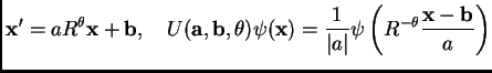
![$\displaystyle W(a,\mathbf{b},\theta)[f] = \int \frac{1}{\vert a\vert} \overline...
... R^{-\theta}\frac{\mathbf{x}-\mathbf{b}}{a} \right) f(\mathbf{x}) d^2\mathbf{x}$](img134.png)
![$\displaystyle W(a,\mathbf{b},\theta)[f] = a \int \exp(\imath \mathbf{b}\mathbf{...
...\hat\psi}\left( a R^{-\theta}\mathbf{k}\right) \hat f(\mathbf{k}) d^2\mathbf{k}$](img135.png)
![\includegraphics[width=100mm]{fig/e10-2001-205/DWT/dec2d.eps}](img145.png)